Cedar walkthrough (from cedar.ipynb)

This page turns cedar.ipynb into a narrative set of worked examples you can copy/paste into your own notebooks or scripts. It focuses on use cases and interpretation of the core metrics:

• COP: coefficient of performance (cooling efficiency)

• SHR: sensible heat ratio (how much cooling is “sensible” vs latent)

• ECOP: effective COP = COP × SHR

• CDD: cooling degree days exceedance

• eCDD: effective CDD = CDD / (COP × SHR) = CDD / ECOP

Note

All temperatures in the APIs below are Kelvin and relative humidity is 0–1.

1) Build an SHR model (humidity sensitivity)

SensibleHeatRatioModel computes SHR from air temperature plus either relative humidity or dew point (it converts dew point → RH internally).

from cedar.metrics.shr import SensibleHeatRatioModel

shr_model = SensibleHeatRatioModel(
    p_atm=101_325.0,
    t_evap_k=273.15,
    approach_temp=1.0,
    C_p=1020.05,
    H_fg=2.501e6,
    rh_out=1.0,
)

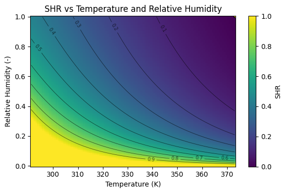
SHR as a function of temperature and relative humidity.

Example: compute a full (T, RH) surface (vectorized).

import numpy as np

temp_axis = np.linspace(283.15, 333.15, 120)   # K
rh_axis   = np.linspace(0.0, 1.0, 100)         # 0–1
temp_grid, rh_grid = np.meshgrid(temp_axis, rh_axis)

shr_grid = shr_model.shr(temp_grid, rh_array=rh_grid)

2) Build a COP model (fast, vectorized)

SingleFluidCOP builds a dense internal lookup once, then interpolates COP quickly for scalars and arrays.

from cedar.metrics.cop import SingleFluidCOP

hp = SingleFluidCOP(
    "R134a",
    t_evap_k=273.15,
    delta_t_cond=10,
    eta_is=0.8,
    delta_t_min=10.0,
)

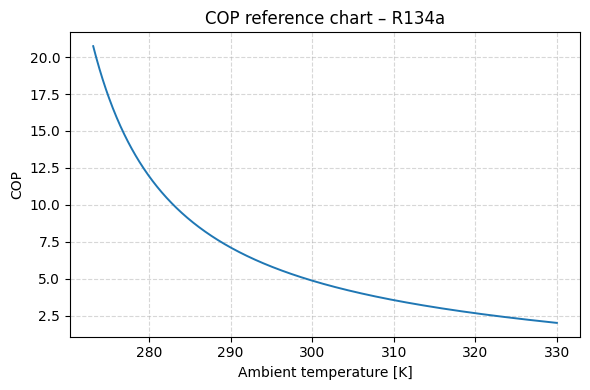
COP reference curve vs ambient temperature for one operating point.

3) Use case: compare system archetypes (refrigerants + operating points)

One way to use CEDAR is to compare “system archetypes” across the same ambient profile (e.g., comfort cooling vs cold storage).

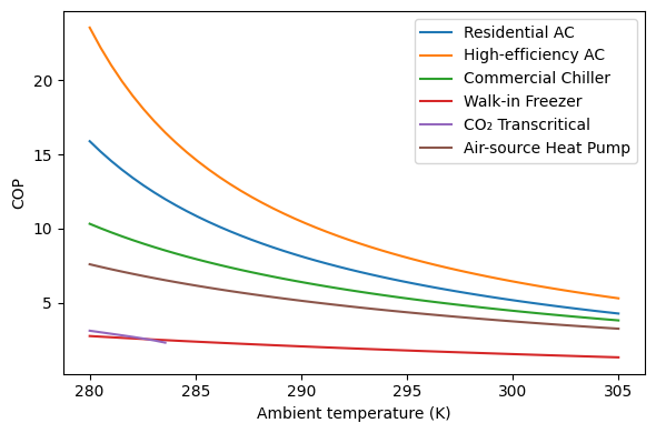
Example COP profiles for multiple refrigerants / operating assumptions.

Skeleton pattern (from the notebook): create a list of configs and loop.

import numpy as np
import matplotlib.pyplot as plt

ambient_profile = np.linspace(280, 305, 50)  # K

configs = [
    dict(label="Residential AC", refrigerant="R410A", t_evap_k=278.15, delta_t_cond=10, eta_is=0.75, delta_t_min=10.0),
    dict(label="High-efficiency AC", refrigerant="R32",   t_evap_k=279.15, delta_t_cond=8,  eta_is=0.80, delta_t_min=8.0),
    dict(label="Commercial Chiller", refrigerant="R134a", t_evap_k=273.15, delta_t_cond=12, eta_is=0.78, delta_t_min=12.0),
    dict(label="Walk-in Freezer",    refrigerant="R404A", t_evap_k=248.15, delta_t_cond=15, eta_is=0.70, delta_t_min=15.0),
]

fig, ax = plt.subplots()
for cfg in configs:
    hp = SingleFluidCOP(
        cfg["refrigerant"],
        t_evap_k=cfg["t_evap_k"],
        delta_t_cond=cfg["delta_t_cond"],
        eta_is=cfg["eta_is"],
        delta_t_min=cfg["delta_t_min"],
    )
    ax.plot(ambient_profile, hp.cop(ambient_profile), label=cfg["label"])
ax.set_xlabel("Ambient temperature (K)")
ax.set_ylabel("COP")
ax.legend()

4) Use case: “effective performance” with humidity (ECOP)

Humidity matters: latent load reduces “useful” cooling capacity. ECOP combines COP and SHR into one metric:

ECOP = COP × SHR

from cedar.metrics.effective_cop import EffectiveCOP

ecop_model = EffectiveCOP(cop_model=hp, shr_model=shr_model)
ecop_grid = ecop_model.ecop(temp_grid, rh_array=rh_grid)

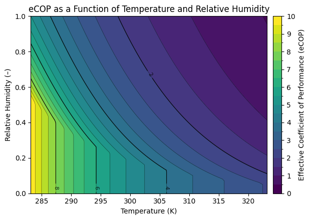
ECOP surface (COP × SHR): efficiency penalized under humid conditions.

5) Use case: CDD and effective cooling demand (eCDD)

CoolingDegreeDays gives exceedance above a base temperature; you can then scale demand by effective performance:

eCDD = CDD / (COP × SHR) = CDD / ECOP

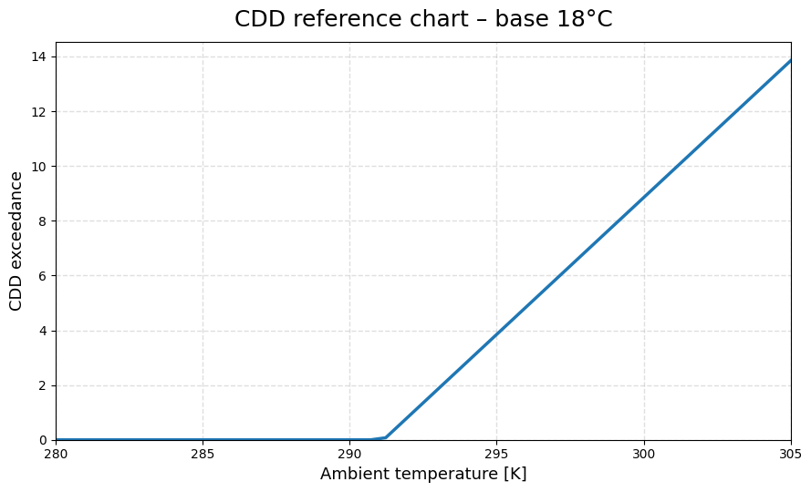
Example CDD exceedance curve for a base temperature of 18°C.

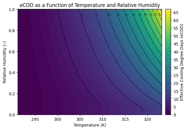
Effective CDD (CDD / ECOP): demand rises with heat and humidity.

Minimal usage:

from cedar.metrics.cdd import CoolingDegreeDays
from cedar.metrics.effective_cdd import EffectiveCDD

cdd_model = CoolingDegreeDays(base_temperature_K=18.0 + 273.15)
ecdd_model = EffectiveCDD(cdd_model=cdd_model, cop_model=hp, shr_model=shr_model)

temps_K = np.array([295.0, 300.0, 305.0])
dewpoint_K = temps_K - 12.0
ecdd_vals = ecdd_model.ecdd(temps_K, dewpoint_array=dewpoint_K)

6) Tips for climate arrays

• All metric entrypoints are vectorized: if your ambient temperature is (lat, lon) or (time, lat, lon), pass it directly.

• Use either rh_array=... or dewpoint_array=... (exactly one) to avoid ambiguous humidity inputs.

• Expect NaN for unphysical states (e.g., too small lift, invalid temperatures).